Class note from Price Theory course.
Consider an individual looks to buy $m$ goods. Let there be nice assumptions:
- Continuous: that consumption can be expressed as $x\in \R^m$.
- (Strictly?) concave utilities.
- Linear budget: $p\cdot x \le \texttt{Budget}$.
Back of (a big) envelope
Let $\mathbf x^H(p, u), \mathbf x^M(p, I)$ be the Hicksian and Marshallian demand functions.
If we focus on one single good $i\in [m]$, and with a tiny abuse of notation, we can write
$$ \begin{align*} & x_i^{H(\bar U, p_{-i})}(p_i) :=x_i^H(p_i, p_{-i}, \bar U)\cr & x_i^{M(I, p_{-i})}(p_i) :=x_i^M(p_i, p_{-i}, I) \end{align*} $$When economists scribble a downward sloping demand curve on a 2D plane, we are basically holding $(\bar U, p_{-i})$ (or $(I, p_{-i})$) fixed and drawing the Hicksian demand curve $D^H:\lbrace (x_i^H(p_i), p_i)\rbrace$ or Marshallian demand curve: $D^M:\lbrace(x_i^M(p_i), p_i)\rbrace$.
Note: when the two demand curves ($x^H_i, x^M_i$) are drawn together, I prefer to imagine that they’re obtained by start from a point $(p_i, x^\star_i(p_i))$ where $ x_i^{H(\bar U, p_{-i})}(p_i) = x_i^{M(I, p_{-i})}(p_i)$. In this way, the fixed utility level (aka purchasing power, how confusing!) $\bar U$ from the Hicksian demand and budget $I$ from the Marshallian demands should corresponds in the way that, under the same price vector (and individual’s utility function), they have the same consumption outcome. Starting from the point $(p_i, x^\star_i(p_i))$ where H/M demand curves cross, we draw them:
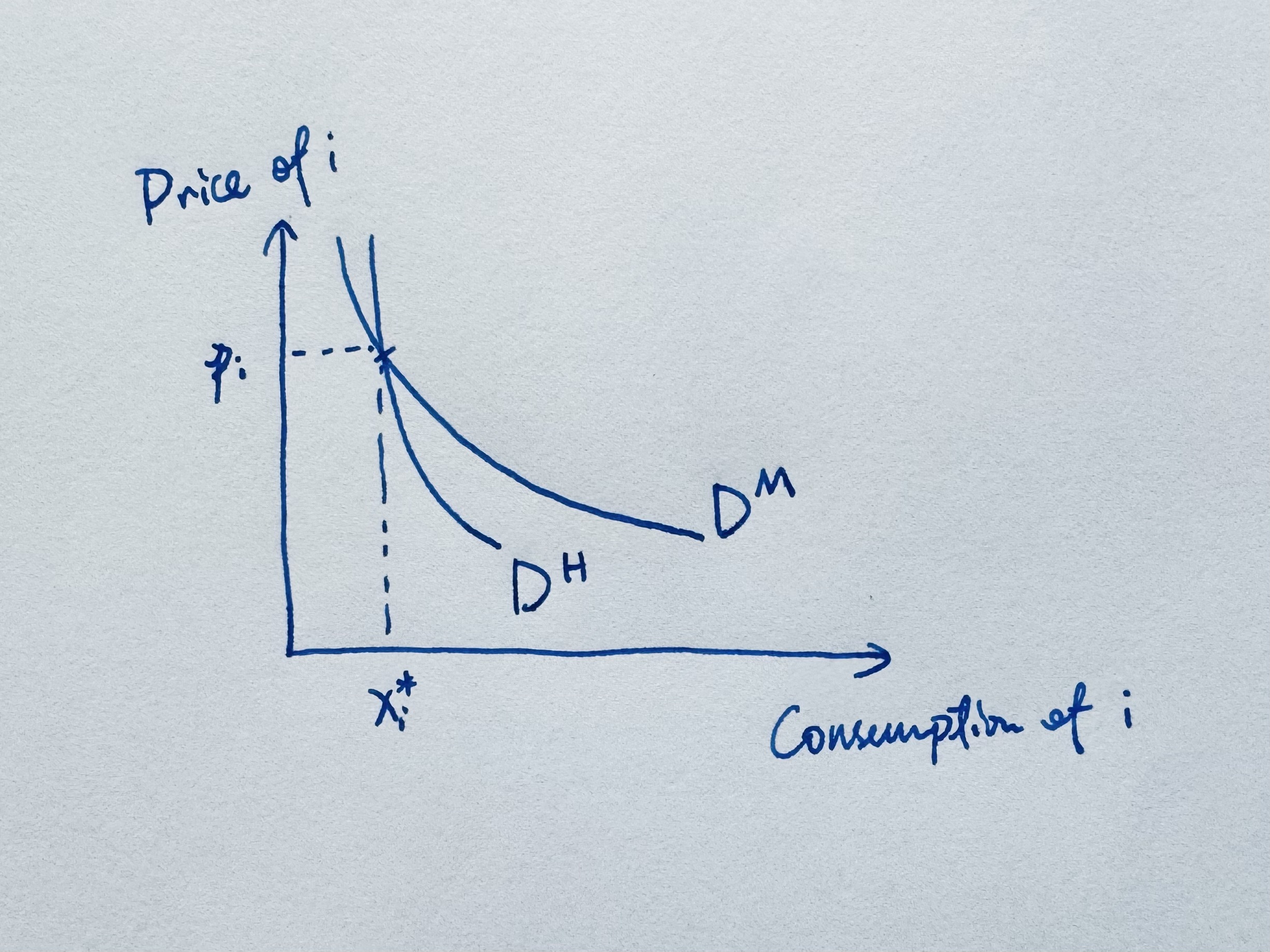
Figure 1. If the Hicksian demand curve is below the Marshallian demand curve, it’s when the income effect around $(p, I)$ is positive: $\partial_I\mathbf x^M(p, I) > 0$.
It’s more intuitive to think about the Marshallian demand, but it’s more mathematically convenient (and precise) to work around the Hicksian demand. Consider when price drops: $p_i \to p_i'$ and we want to measure the utility gain of the individual. Hicksian demand changes to $x_i^H(p_i')$. Denote the Hicksian demand’s expenditure function as
$$ e(p, \bar U):=\min_x\lbrace p\cdot x:U(x)\ge \bar U\rbrace. $$The expenditure function measures how many dollars the individual need to reach utility level $u$ at prices $p$. Therefore, the change in the expenditure function can be interpreted as the exact monetary measure of the utility change due to that price variation. Now, by the envelope theorem (Shephard’s Lemma):
$$ \frac{\partial e(p,u)}{\partial p_i} = x_i^H(p,u). $$We have
$$ e(p_i, p_{-i},\bar U) - e(p_i', p_{-i},\bar U) = \int_{p_{i}'}^{p_i} x_i^{H(p_{-i},\bar U)}(s)ds. $$Thus, the area under the Hicksian demand curve gives the change in the minimum expenditure required to hold utility constant, i.e., the exact monetary measure of the utility change due to that price variation.
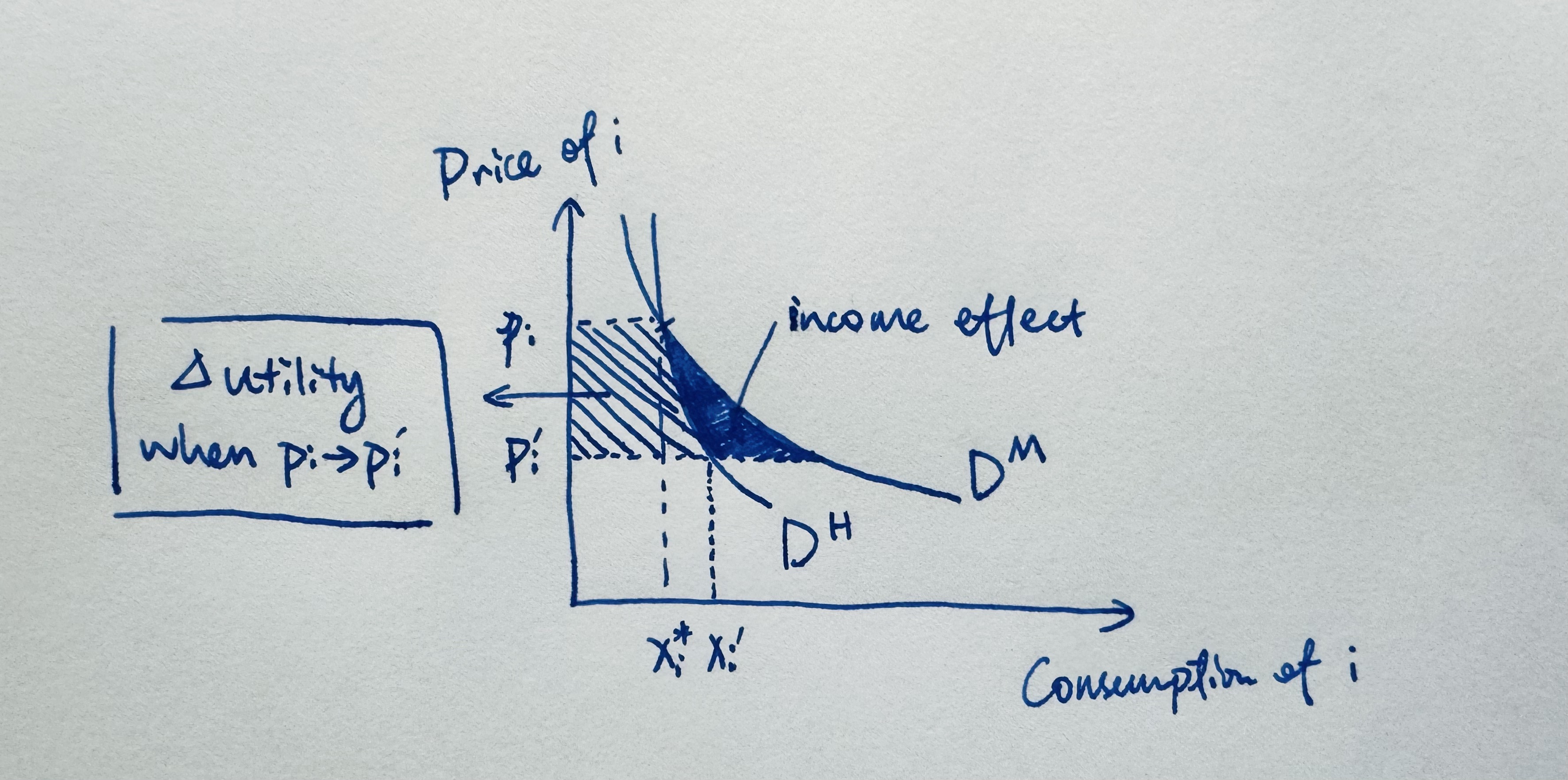
Figure 2. The Hicksian area is the the exact monetary measure of the utility change due to price change. The Marshallian area is corrupted by income effect.
Similarly, let’s consider when at price $x_i^\star$ is optimal purchase for $p_i$, but the individual mistakenly buys more, $x_i' > x_i^\star$. The shaded areas w.r.t. the Hicksian demand curve:
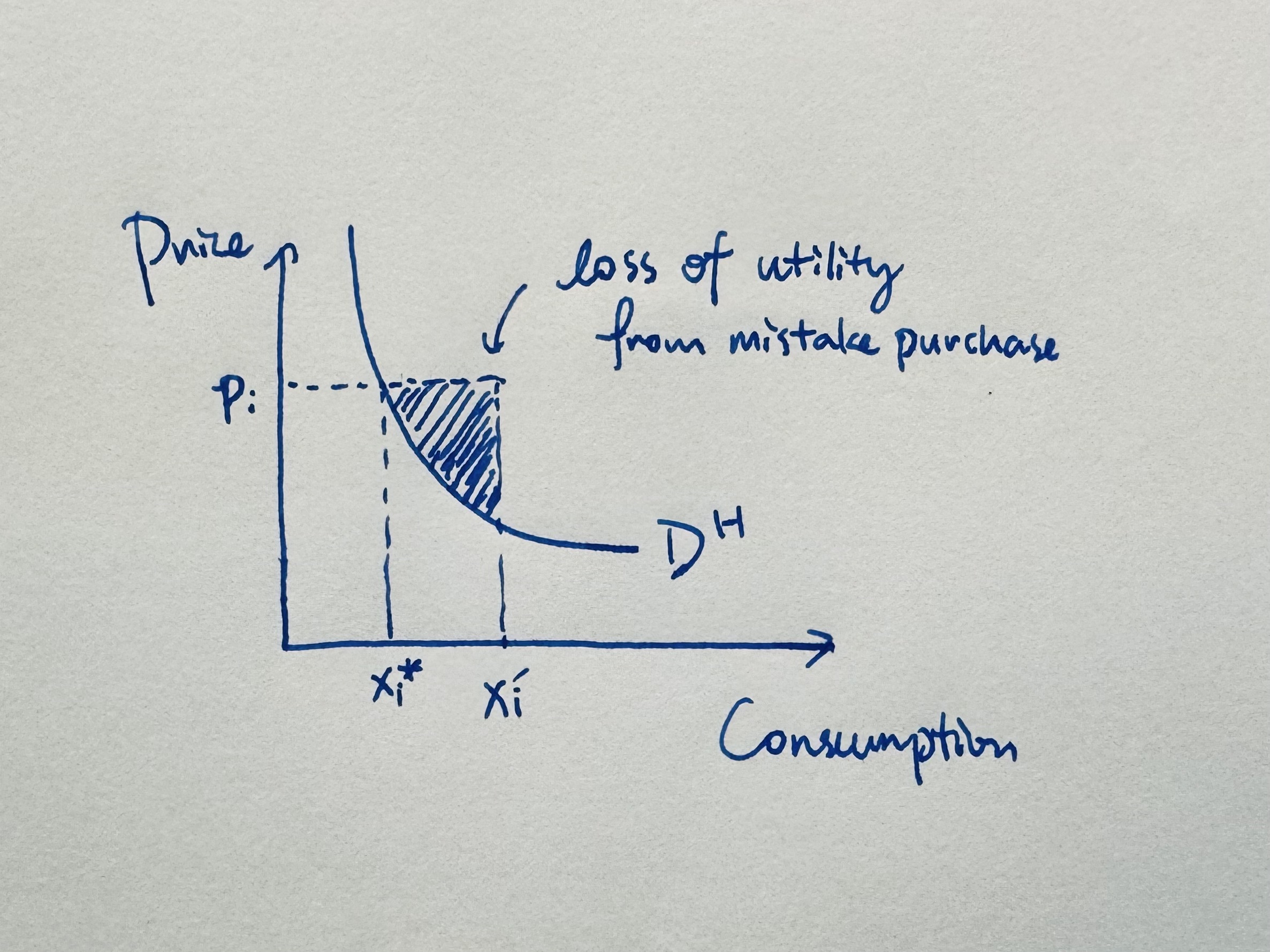
Figure 3.
is the utility loss (measured in money) from being mistakenly buying $x_i'$ when best option is $x_i^\star$. Beacuse on the Hicksian demand curve each point $(x_i, p_i^H(x_i))$ corresponds precisely to the marginal willingness to pay for that quantity, by construction. So, utility loss can be measure as the following intergration:
$$ \text{Utility loss in Money} = \int_{x^\star_i}^{x_i'} [p^H(x) - p_i]\ \text{d}x. $$Now let’s wave our hand
It’s all about tradeoffs — in economic analysis, a little concession in rigorous gives back a lot more for intuition.
So, let’s assume income effect is negligible (e.g. small price changes or quasi-linear utility), we can then use Marshallian demand curve as a substitute of the Hicksian demand curve to approximately measure the change in individual’s utility as price goes down or up, or when individual’s purchase goes wrong.
In other words, we assume a downward sloping demand curve, and we don’t really care about the income effect and don’t differentiate whether it’s Marshallian or Hicksian.
Two interesting conclusions then arise:
Advertisement
Suppose the seller of product $i$ want to increase their sales from $x_i^\star \to x_i'$ when price is $p_i$. One way he can do it is by lowering price to $p_i'$. In this way, he gains $p_i'x_i' - p_ix_i$, which (approximately) corresponds to $S - T$ (Figure 3.1):
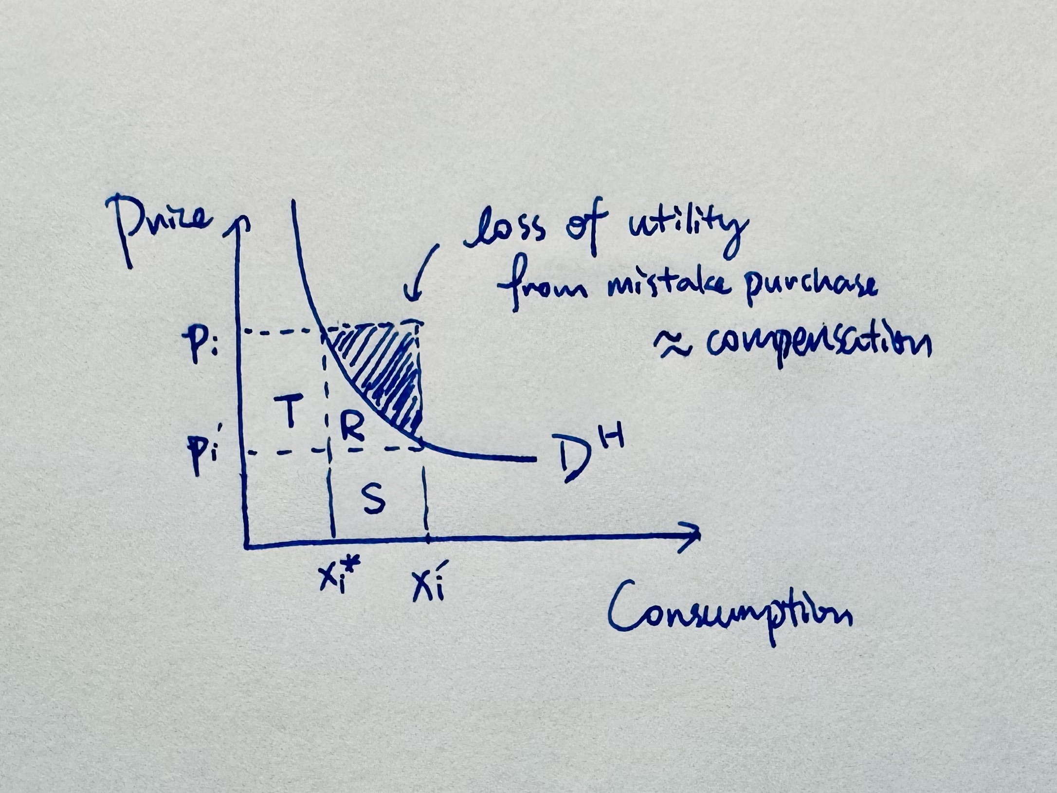
Figure 3.1 Note that $D^H$ should eh, be both the Marshallian demand and the Hicksian demand.
That’s one way. But let’s think outside the box. Let’s say, instead of lowering the price, the seller compensate the consumer an amount of money to buy $x_i'$, which is an undesirable amount if price is $p_i$. Let the compensation be equal to the area of the shade (Figure 3.1)—this amount would exactly makes up the utility loss of the individual who consume $x_i'$ instead of $x_i^\star$ at price $p_i$. In this way, the seller increase sales to $x_i'$ while maintaining price $p_i$ and losing the revenue of the shaded area. In this way, seller’s utility increment is $S + R$. So the seller gets jigher revenue :)
In fact, $S + R$ can be MUCH bigger than $S - T$ if you consider the price and demand changes are small — then $S + R$ would dominate $S - T$ with an order.
I think this is perhaps the most minimalistic elegant justification for the advertisement industry!
A side argument also tells something about shopping: you don’t lose a lot when you buy too much! (only the triangular shaded area) But you’re a moron if you buy expensive. We call them 水鱼.
Loss of insufficient information (deceptions), and regulation
Let’s say the seller lies about product $i$’s quality. The demand curve under fake info is $D'$ would lies above the true demand curve.
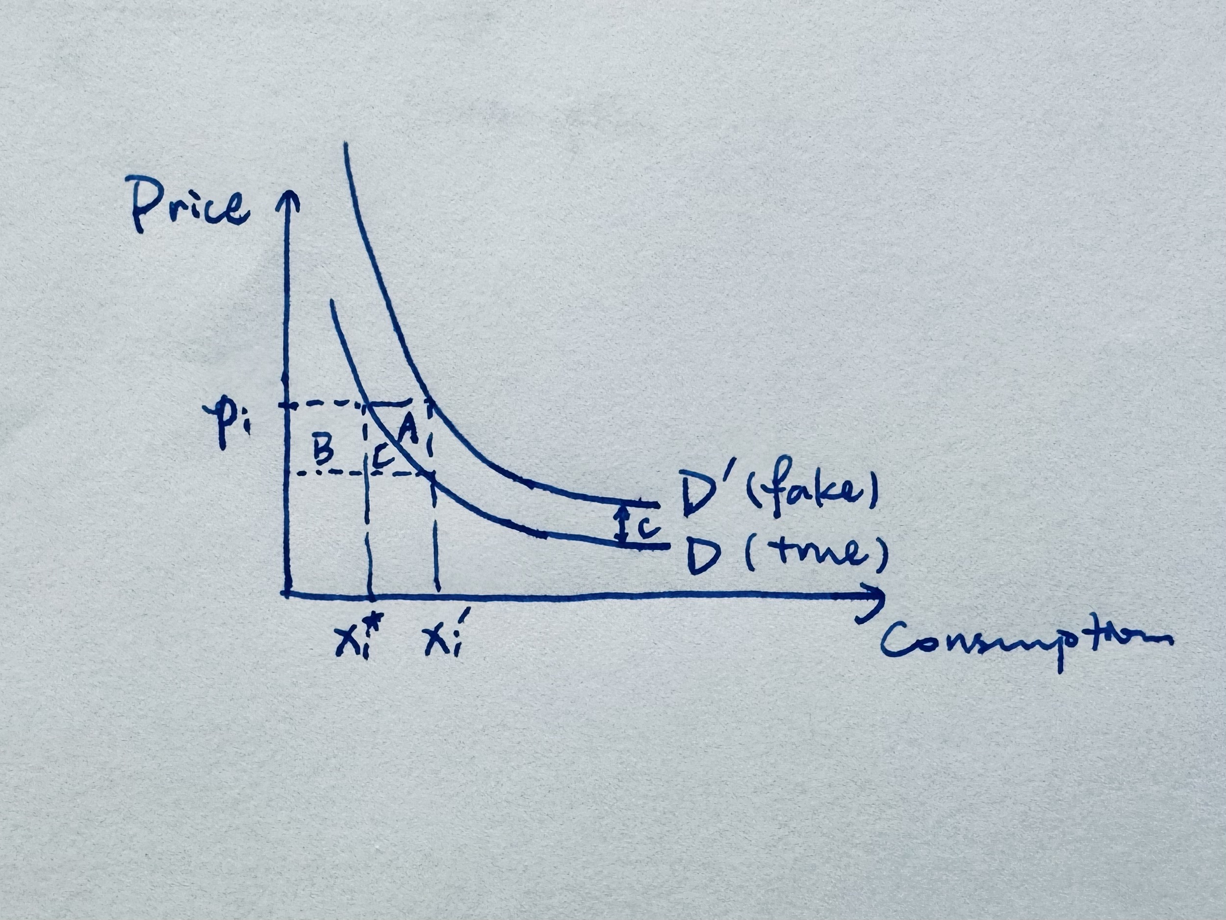
Figure 4. Assumption DD: these two demand curves’ vertical gap is constant $p'(x_i) - p(x_i) \equiv c, \forall x_i$.
Under the lie, when the product’s really crappy but individuals buy more than they should: $(x_i', p_i)$. A regulator can either
Force the seller to tell the truth. Then the individual goes back to buy $x_i^\star$ and the utility gain from resolving the truth of the product is area $A$ (Figure 4).
However, if the seller is forced to increase his product quality so that it supports $D'$. Then individuals now really are happy to buy $x_i'$ amount under price $p_i$, and the utility gain would equal to the area $B + C$ (Figure 4).
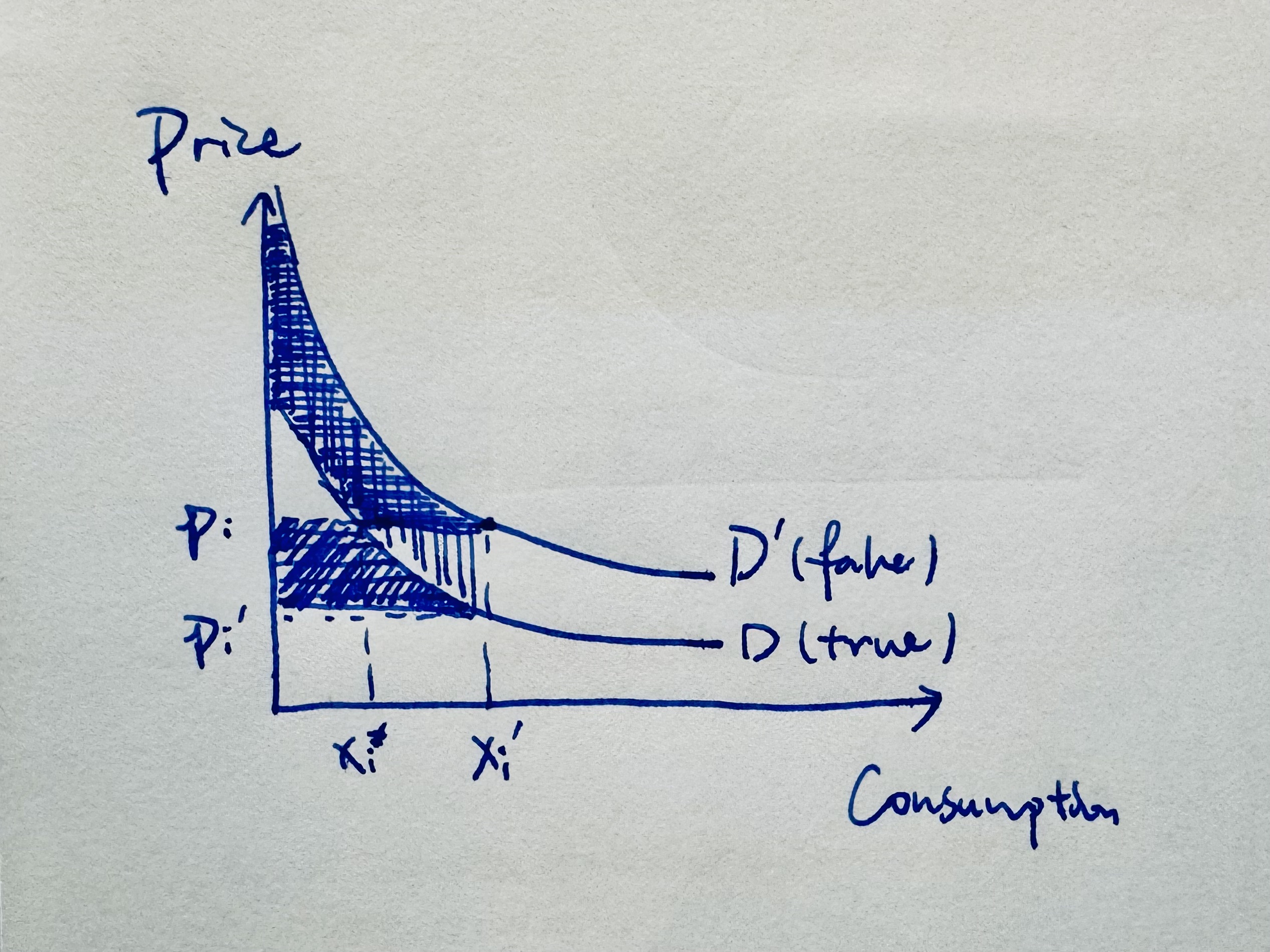
Figure 4.1 The utility gain from increasing product quality so that demand curve $D$ move to $D'$, is equal to area $B+C$ (Figure 4) under Assumption DD that the demand curves’ vertical gap is constant.